Contrastive Learning

Understanding how CLIP learns visual-semantic embeddings through contrastive loss

Contrastive Learning in CLIP

Contrastive learning is the training methodology that enables CLIP to learn aligned visual and semantic representations. The key insight: maximize agreement between matched image-text pairs while minimizing agreement between mismatched pairs.

Core Concept

Given a batch of N (image, text) pairs:

1. Encode all images → N image embeddings
2. Encode all texts → N text embeddings
3. Compute N×N similarity matrix
4. Train to maximize diagonal (correct pairs) and minimize off-diagonal (incorrect pairs)

Symmetric Loss: CLIP computes loss from both image→text and text→image directions, ensuring bidirectional alignment.

The Contrastive Loss Function

OpenCLIP implements the contrastive loss in src/open_clip/loss.py. The core loss is a symmetric cross-entropy loss over the similarity matrix.

Implementation

From src/open_clip/loss.py:68-155:

class ClipLoss(nn.Module):
    def forward(
            self,
            image_features,
            text_features,
            logit_scale,
            logit_bias=None,
            output_dict=False,
    ):
        device = image_features.device
        
        # Compute similarity matrix (N×N)
        logits_per_image, logits_per_text = self.get_logits(
            image_features,
            text_features,
            logit_scale,
            logit_bias=logit_bias,
        )

        # Ground truth: diagonal matrix (i-th image matches i-th text)
        labels = self.get_ground_truth(device, logits_per_image.shape[0])

        # Symmetric cross-entropy loss
        total_loss = (
            F.cross_entropy(logits_per_image, labels) +
            F.cross_entropy(logits_per_text, labels)
        ) / 2

        return {"contrastive_loss": total_loss} if output_dict else total_loss

Logits Computation

From src/open_clip/loss.py:104-130:

def get_logits(self, image_features, text_features, logit_scale, logit_bias=None):
    if self.world_size > 1:
        # Gather features from all GPUs for large batch sizes
        all_image_features, all_text_features = gather_features(
            image_features,
            text_features,
            ...
        )
        logits_per_image = logit_scale * all_image_features @ all_text_features.T
        logits_per_text = logit_scale * all_text_features @ all_image_features.T
    else:
        # Single GPU: compute scaled cosine similarity
        logits_per_image = logit_scale * image_features @ text_features.T
        logits_per_text = logit_scale * text_features @ image_features.T

    if logit_bias is not None:
        logits_per_image += logit_bias
        logits_per_text += logit_bias

    return logits_per_image, logits_per_text

Mathematical Formulation

Given normalized embeddings I (images) and T (texts):

Similarity Matrix

S = τ · I · T^T

Where:

• τ (tau) = logit_scale.exp() - learnable temperature parameter
• S[i,j] = scaled cosine similarity between i-th image and j-th text

Loss Function

L = 1/2 * [L_i2t + L_t2i]

L_i2t = -1/N * Σ log(exp(S[i,i]) / Σ_j exp(S[i,j]))  # Image to text
L_t2i = -1/N * Σ log(exp(S[i,i]) / Σ_j exp(S[j,i]))  # Text to image

This is equivalent to cross-entropy loss with ground truth labels on the diagonal.

Visual-Semantic Embedding Space

Contrastive learning creates a joint embedding space where:

Positive Pairs (Matching)

• Image of “a dog playing fetch” ↔ Text “a dog playing fetch”
• Model learns to embed these close together
• High cosine similarity (→ 1.0)

Negative Pairs (Mismatched)

• Image of “a dog playing fetch” ↔ Text “a cat sleeping”
• Model learns to embed these far apart
• Low cosine similarity (→ 0.0 or negative)

Emergent Properties

Through large-scale contrastive training:

1. Semantic clustering - Similar concepts cluster together
2. Cross-modal alignment - “dog” (text) aligns with dog images
3. Compositional understanding - Model learns objects, actions, attributes
4. Zero-shot transfer - Embeddings generalize to unseen concepts

Training Objective and Batch Construction

In-Batch Negatives

CLIP uses an efficient strategy: in-batch negatives

• Batch size N creates N positive pairs
• Each pair has (N-1) negative examples from other samples
• Total comparisons: N² (N positive + N(N-1) negative)

Large batch sizes are critical for contrastive learning. More negatives = better training signal. OpenCLIP supports batch sizes up to 100K+ across distributed GPUs.

Batch Construction Example

Given batch size N=4:

Images:    [img0, img1, img2, img3]
Texts:     [txt0, txt1, txt2, txt3]

Similarity Matrix (4×4):
        txt0  txt1  txt2  txt3
img0  [HIGH   low   low   low ]  ← img0 matches txt0
img1  [ low  HIGH   low   low ]  ← img1 matches txt1
img2  [ low   low  HIGH   low ]  ← img2 matches txt2
img3  [ low   low   low  HIGH ]  ← img3 matches txt3

Goal: Maximize diagonal, minimize off-diagonal

Ground Truth Labels

From src/open_clip/loss.py:91-102:

def get_ground_truth(self, device, num_logits) -> torch.Tensor:
    # Ground truth: each image i should match text i
    labels = torch.arange(num_logits, device=device, dtype=torch.long)
    
    if self.world_size > 1 and self.local_loss:
        # Adjust labels for distributed training
        labels = labels + num_logits * self.rank
        
    return labels

Labels are simply [0, 1, 2, ..., N-1] - each sample matches its corresponding index.

Advanced Training Techniques

Local Loss

For distributed training, compute loss locally on each GPU to save memory:

if self.local_loss:
    # Only compute gradients for local image features
    logits_per_image = logit_scale * image_features @ all_text_features.T
    logits_per_text = logit_scale * text_features @ all_image_features.T

Reduces space complexity from O(n²) to effectively O(n).

Gather with Gradient

Enable gradient flow during all-gather operation:

if gather_with_grad:
    all_image_features = torch.cat(torch.distributed.nn.all_gather(image_features))
    all_text_features = torch.cat(torch.distributed.nn.all_gather(text_features))

Allows backpropagation through distributed features.

SigLIP Loss (Alternative)

OpenCLIP also implements SigLIP loss from src/open_clip/loss.py:330-464:

class SigLipLoss(nn.Module):
    """ Sigmoid Loss for Language Image Pre-Training (SigLIP) 
    Uses sigmoid instead of softmax for better scaling.
    """
    def _loss(self, image_features, text_features, logit_scale, logit_bias=None):
        logits = self.get_logits(image_features, text_features, logit_scale, logit_bias)
        labels = self.get_ground_truth(...)
        loss = -F.logsigmoid(labels * logits).sum() / image_features.shape[0]
        return loss

Benefits:

• Better scaling to very large batches
• No softmax normalization overhead
• Independent per-pair loss computation

Training Configuration

Example training with contrastive loss:

python -m open_clip_train.main \
    --train-data="/data/laion400m/{00000..41455}.tar" \
    --batch-size=256 \
    --epochs=32 \
    --model=ViT-B-32 \
    --local-loss \        # Enable local loss for memory efficiency
    --gather-with-grad    # Enable gradient gathering

Key Hyperparameters

• Batch size: Larger = more negatives = better training (256-32K typical)
• Learning rate: 5e-4 to 1e-3 typical for CLIP
• Warmup: Gradual learning rate increase (2000-10000 steps)
• Temperature (τ): Learned, initialized to ~2.66

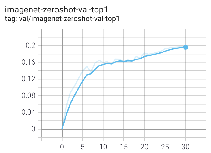
Loss Curves

During training, monitor:

1. Contrastive loss - Should decrease steadily
2. Accuracy - Top-1/Top-5 on diagonal predictions
3. Zero-shot metrics - Periodic ImageNet zero-shot evaluation

From the README:

When run on a machine with 8 GPUs the command should produce the following training curve for Conceptual Captions

Reference Implementation

Key files:

• src/open_clip/loss.py - ClipLoss, SigLipLoss, CoCaLoss implementations
• src/open_clip/model.py:265-480 - CLIP model with forward pass
• src/open_clip_train/train.py - Training loop

Related Concepts

CLIP Overview

High-level architecture and design principles

Zero-Shot Classification

How contrastive embeddings enable zero-shot inference

Further Reading

• Original CLIP Paper: Learning Transferable Visual Models From Natural Language Supervision
• SigLIP Paper: Sigmoid Loss for Language Image Pre-Training
• OpenCLIP Scaling Laws: Reproducible scaling laws for contrastive language-image learning